Help
This page describes different features of the web server and provides some theoretical background. For a quick hands-on manual please see Tutorial. Technical documentation of the algorithm of chromatin 3D structure folding is available here, and the algorithm description of spatial chromatin architecture alteration by structural variations is available here.
- Introduction
- Modelling overview
- Browsing data
- Running a simulation
- Submitting custom data
- Modelling parameters
- Modelling guidelines and common pitfalls
- Limitations of 3D structure modelling method
- SV-driven alterations of chromatin spatial architecture
- Running time of simulation
- FAQ
Introduction
Web server consists of 2 main tools: modelling pipeline, accessible via New request form, and an interactive data browser (available here).
To start modelling you can go directly to the Request form and send a new request. In the simplest case, when the default dataset and modelling parameters are used all you need to do is to specify a genomic region you are interested in. In a more advanced scenario you may want to play with modelling parameters or to provide your own data.
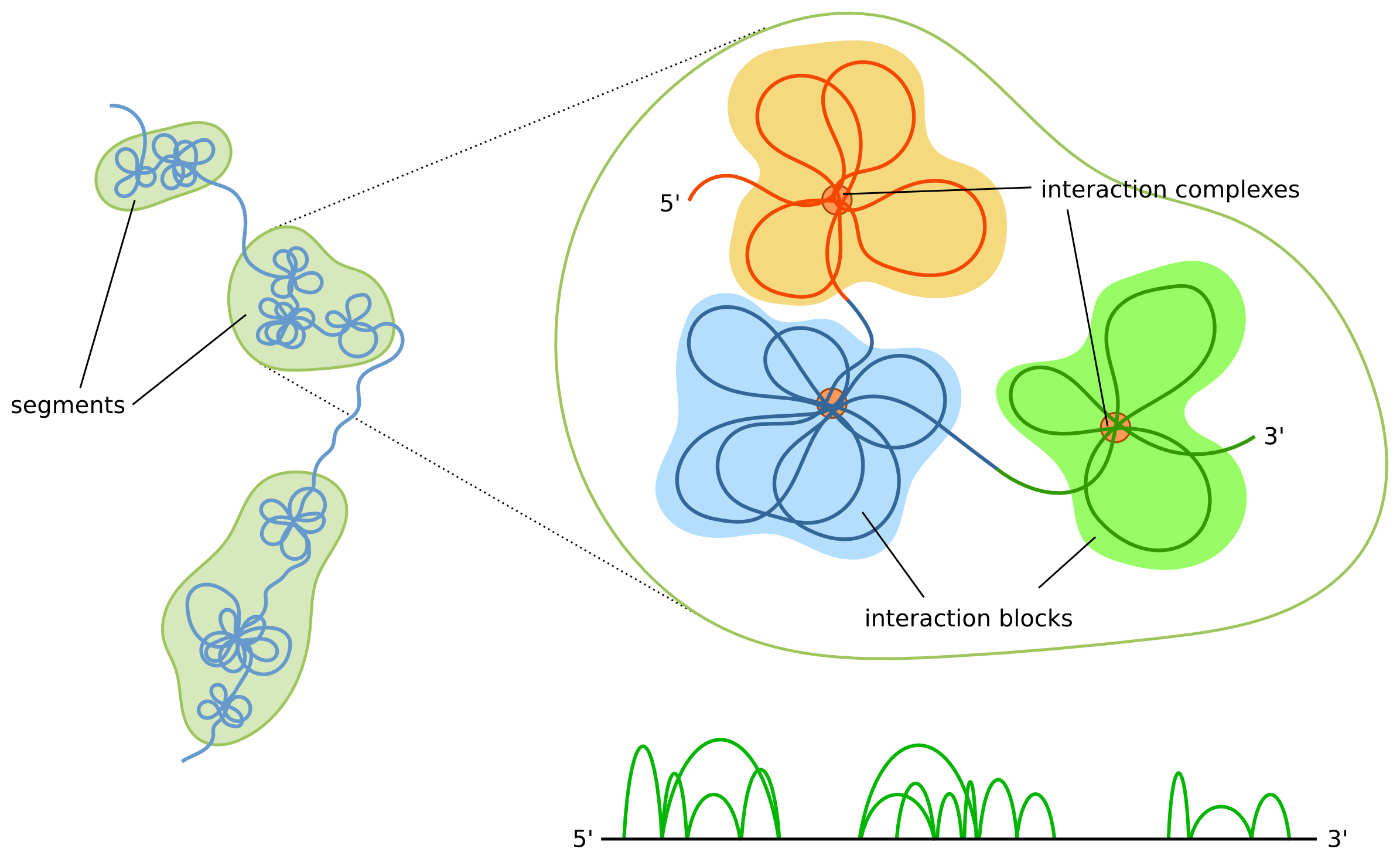
The shape of the modelled structures is dependent not only on the interactions data itself, but also on the boundaries of the segments. The most prominent features of our model are interaction complexes which form characteristic "clumps" of chromatin loops. Simplifying things a bit, each segment will form a separate clump. Thus, if a region consists of only a few segments then it will be represented as a small number of large clumps, as opposed to multi-segment regions, which will consist of a large number of smaller clumps. Additionally, the higher number of segments the higher the chromatin chain flexibility will be. Because of these reasons users are encouraged to inspect segment boundaries before running the simulations. A data browser can be used for visual inspection and possible adjustments.
With 2.0 version of 3D-GNOME, users gain the ability to predict structural variation-driven changes in 3D conformations of specific loci in human genome. In the default settings, 3D-GNOME 2.0 employs chromatin interaction paired-end tag sequencing (ChIA-PET) data for the GM12878 cell line (6) as the reference chromatin interaction map and sets of structural variants (SVs) emerging across human populations constructed by The 1000 Genome Project (Phase 3) as the source of genetic variation. When relying on our precomputed reference 3D model, users may also provide a particular custom SVs. 3D-GNOME 2.0 returns both the reference 3D structure and the structure modified by SVs. Alternatively, users can submit their list of loops obtained from 3C based methods such as Hi-C or ChIA-PET (interaction file format is explained here) and a custom SV list and generate 3D structures of their loci and genomes of choice. Example of SV list in VCF format is available here and results of the simulation based on that particular SV list within TAL locus (chr1:47656996-48192898) are available here.
For simulation you can select CTCF-mediated interactions only, or both CTCF- and RNAPII-mediated interactions at the same time
Modelling overview
Our 3D structure modelling is based on the topological domains and chromatin loops which constitute the basic units on the genome organization. We use a hierarchical approach, in which we first model the low-resolution structure (where every bead corresponds to approximately megabase-sized regions) reflecting the relative placement of the domains, and then we use it to guide the high-resolution modelling in which chromatin loops are shaped (here every bead corresponds to anything from a few kb to tens or hundred of kb long chromatin fiber, depending on the region).
Topological domains are regions with abundant interactions throughout the region and substantially fewer interactions with other regions (ie. loci within a domain tend to interact with each other rather then with loci located in other domains). While domains appear as clearly discernable blocks along the diagonal of a Hi-C or ChIA-PET heatmaps there is no agreement as to their precise definition - different studies report different number of identified domains depending, among the others, on the sequencing coverage and domain calling algorithm.
The term "topologically associating domains" (TADs) is usually used in the context of Hi-C technique, while for ChIA-PET a "chromosome contact domains" (CCDs) is used. CCDs differ from TADs in the way they are defined - TADs are defined based on the Hi-C heatmaps (which aggregates all the Hi-C interactions), and CCDs are based on PET clusters solely. Our algorithm is independent from a specific method and can work for any type of regions, and to make it clear (and to highlight the distinction between the biological domains and the corresponding computational object) we will use a term "segments" to denote domains.
We base our approach on ChIA-PET data, where one can distinguish PET clusters, strong interactions that appear multiple times in the dataset, and which are anchored at the binding peaks, and singletons, which correspond to weak interactions. In principle, one can use any experimental technique that captures the genome-wide interactions between different loci, as long as a distinction between weak and strong interactions can be made. Particularly, Hi-C data can be used - in that case loop calling should be performed and the identified loops would be treated as a strong interactions, whereas the remaining contacts would be treated as weak ones.
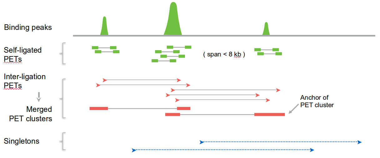
The main idea of the algorithm is to identify the segments (we use strong interactions for that, but one can use also weak ones or any other data source) and model their spatial locations using heatmaps obtained from aggregating weak interactions, and then model all segments sequentially based on the strong interactions
Browsing data
You can browse either the default dataset (for that please select cell line and chromosome from the list, and click on the "Load" button), or your own data - simply select a file after clicking on the "Browse" button. The file should be in bedpe-like format described here.
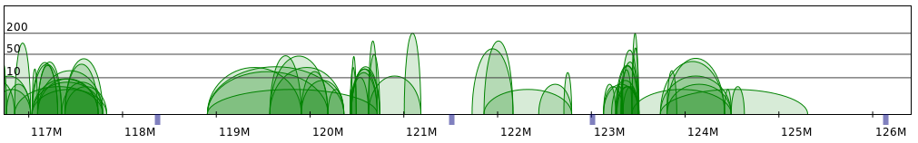
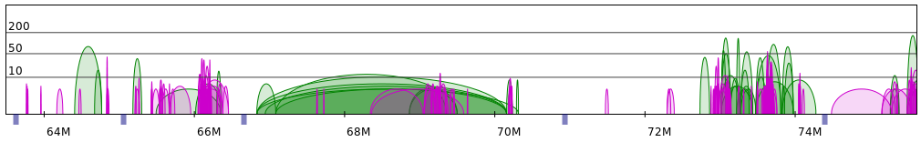
After the dataset is loaded an interaction plot will appear (similar to the one presented on Fig 1. Please note that due to presentation reasons we only display interactions shorter than 5Mb). You can control the plot interactively using a mouse (details below). An important feature of the tool is the possibility to create a segment split, which can be later exported to a text file and used when submitting a request. Segments boundaries are marked with blue rectangles. To add a new boundary left-click anywhere in the boundary markers area. You can click-and-drag boundary markers to move them to a desired location. To remove an existing boundary right-click on it.
Rather than create a split from scratch you can use the automatic splitting tool which makes the split based on the size of gaps between interaction networks and relative segment sizes (this feature only works for uploaded data, for the default dataset our current, manually adjusted split is presented). You are strongly advised to visually inspect the split to make sure it is reasonable.

Mouse controls:
- Use mouse wheel to zoom in and out. Currently selected region is marked by the sliding box.
- You can use click'n'drag technique to move the sliding window and change the displayed region.
- You can also click anywhere on the sliding bar to move there instantly.
Running a simulation
In the simplest mode to run the simulations one only needs to specify the genomic region. In this case a default dataset (see this FAQ question for details) and modelling parameters are used. For a description of sample results please see Tutorial.
Submitting custom data
Interaction files
You can run the simulation using your own data. You need to provide 2 files, for strong and weak interactions.
While our modelling was designed specifically for the ChIA-PET in principle you can use any source of interaction frequency data, as long as you can identify weak and strong interactions.
For the interaction files we use a custom data format similar to the bedpe format used by BEDTools (see specification), which was in turn based on the bed format of the UCSC Genome Browser (see specification). The format is as follows:
chr1 start1 end1 chr2 start2 end2 orientation1 orientation2 score factorwhere
- chr1 - id of the chromosome on which the first end of the interaction is located, eg. "chr1", "chr14", "chrX",
- start1 - starting position of the first interaction end,
- end1 - ending position of the first interaction end,
- chr2 - id of the chromosome on which the first end of the interaction is located, eg. "chr1", "chr14", "chrX",
- start2 - starting position of the second interaction end,
- end2 - ending position of the second interaction end,
- orientation1 - orientation of CTCF motif for first anchor: "L"-left, "R"-right or "N"- not-known; for RNAPII anchors: “N”
- orientation2 - orientation of CTCF motif for first anchor: "L"-left, "R"-right or "N"- not-known; for RNAPII anchors: “N”
- score - value denoting the strength of the interaction,
- factor - name of the factor the interaction was mediated by.
For example, following is an extract from the default dataset:
chr14	35696377	35701390	chr14	36155560	36158360	R	L	8	CTCF
chr14	35696377	35701390	chr14	35879425	35884385	R	L	58	CTCF
chr14	35873369	35878522	chr14	36155560	36158360	N	L	17	CTCF
chr14	35873369	35878522	chr14	35888768	35893204	N	L	7	CTCF
chr14	35879425	35884385	chr14	36155560	36158360	L	L	11	CTCF
chr14	35879425	35884385	chr14	35888768	35893204	L	L	15	CTCF
chr14	35888768	35893204	chr14	36155560	36158360	L	L	29	CTCF
chr14	35451278	35451839	chr14	35509517	35509958	N	N	5	RNAPII
chr14	35344475	35344980	chr14	35873276	35874186	N	N	5	RNAPII
chr14	35610144	35610460	chr14	35869155	35870134	N	N	5	RNAPII
chr14	35723160	35723372	chr14	35868295	35868518	N	N	4	RNAPII
chr14	35753413	35755152	chr14	35763084	35764361	N	N	12	RNAPII
Segment splits
Segment definition should be stored in a tab-delimited BED file (detailed description available here) containing locations of segment splits. The format is as follows:
chr start endwhere
- chr - id of the chromosome, eg. "chr1", "chr14", "chrX",
- start - location of the segment boundary
- end - this value is ignored (but it needs to be present).
A sample excerpt from the default dataset (note that here the third column is identical to the second, but this is an arbitrary choice):
chr1 1634152 1634152
chr1 3735966 3735966
chr1 6072764 6072764
chr1 8966211 8966211
chr1 11059337 11059337
chr1 13354769 13354769
chr1 16818853 16818853
chr1 20011431 20011431
chr1 20994644 20994644
chr1 23774789 23774789
Modelling parameters
For clarity we group the options in sections corresponding to the ones present in the request form.
- General
- Steps number
- CTCF motifs
- Frequency distance scaling
- Count distance scaling
- Genomic distance scaling
- Anchor heatmaps
- Subanchor heatmaps
General
- Use 2D - this allows to restrict the modelling to 2 dimensions. It may be useful when studying the effect of different parameters on the structure.
- Beads per loop - each chromatin loop is represented using a pre-specified number of beads that are
positioned equidistantly between the anchors. The higher the number the shorter genomic regions
the beads correspond to, and the more complex shapes the loop can possibly take.

Different number of beads per loops - Segment definition - this option allows user to submit a file with a custom segment split and effectively control the size of the domains. Details can be found in the Submitting custom data section.
Steps number
These options allows to set the number of simulation iterations performed on every level independently. Large number of simulations may lead to better structures, but at the cost of longer time required for the simulation. In a typical usage one may want to run the simulation using a single iteration on every level (which is done by default) which allows to quickly produce the structure and adjust the simulation parameters if needed. When the parameters seem to have proper values a simulation with a larger number of iterations may be used in order to obtain final structure. Usually 5 to 10 iterations should be sufficient, and the improvement of further increasing this number is not significant.CTCF motifs
These options can be used to decide whether the CTCF motifs orientation should be considered in the modelling and what should be their weight in the overall energy function. The picture presents 2 different shapes of loops depending on the relative motifs orientation (left) and the effect of including CTCF motifs in the modelling on the output structures (right; structures are limited to 2D for clarity).
Frequency - distance scaling
On a segment level a power law relation is used to model the relation between interactions frequency and physical distance. Scale is used to linearly scale the resulting distances. If the structure you obtain from the modelling is too dense (eg. CCDs overlap each other) or too sparse (CCDs are connected by long stretches of chromatin) then you may want to decrease or increase this value. It is also possible to adjust the exponent used (Power setting). A choice of proper value is problematic, as studies suggest that different chromosomal regions are characterized by different scalings. In the current version of the web server it is not possible to accommodate for that and to assign different scalings for different regions.PET count - distance scaling
For the distances between anchors an exponential relation is assumed. To our knowledge there is a lack of experimental data on this level, so we decided to take a very general functional form. It should be noted, however, that these parameters does not play a significant role on the resulting structure, as the distances between anchors are much smaller than the size of chromatin loops. Thus, in a final structure the precise positions of anchors and their relative arrangements are often indiscernible. These settings may be useful for example to create schematic representations of short regions, for example single segments, which may provide a quick overview of the inter-anchor interactions frequency. Base denote the minimal possible distance between anchor beads, hence changing this value influence mostly the closest anchors. Scale can be used to proportionally increase or decrease all the distances. Power and Shift can be used to model the relation more precisely - the former control the non-linear change of distance for different PET count values, and the latter can be used to "shift" this relation - this can be used to make the differences between small PET count values less or more prominent (the higher the value, the less prominent the difference will be).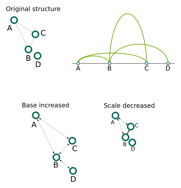
Genomic distance scaling
These parameters describe the relationship between genomic and physical distances which is used on the subanchor level. Intuitively, they control the size of the chromatin loops. By changing the Scale we can change the size of all the loops by the same factor, while Power allows to change the non-linear relationship. A value of 1 means that the relation is linear, ie. if the genomic distance between beads A and B would be 2 times larger, then the physical distance between them should also be 2 times larger. Note that while the loops change their size, the interaction complex remains the same - this is so because the anchors are positioned first, and are kept fixed during the subanchor level modelling. Base is used to enforce a minimal size of the loop.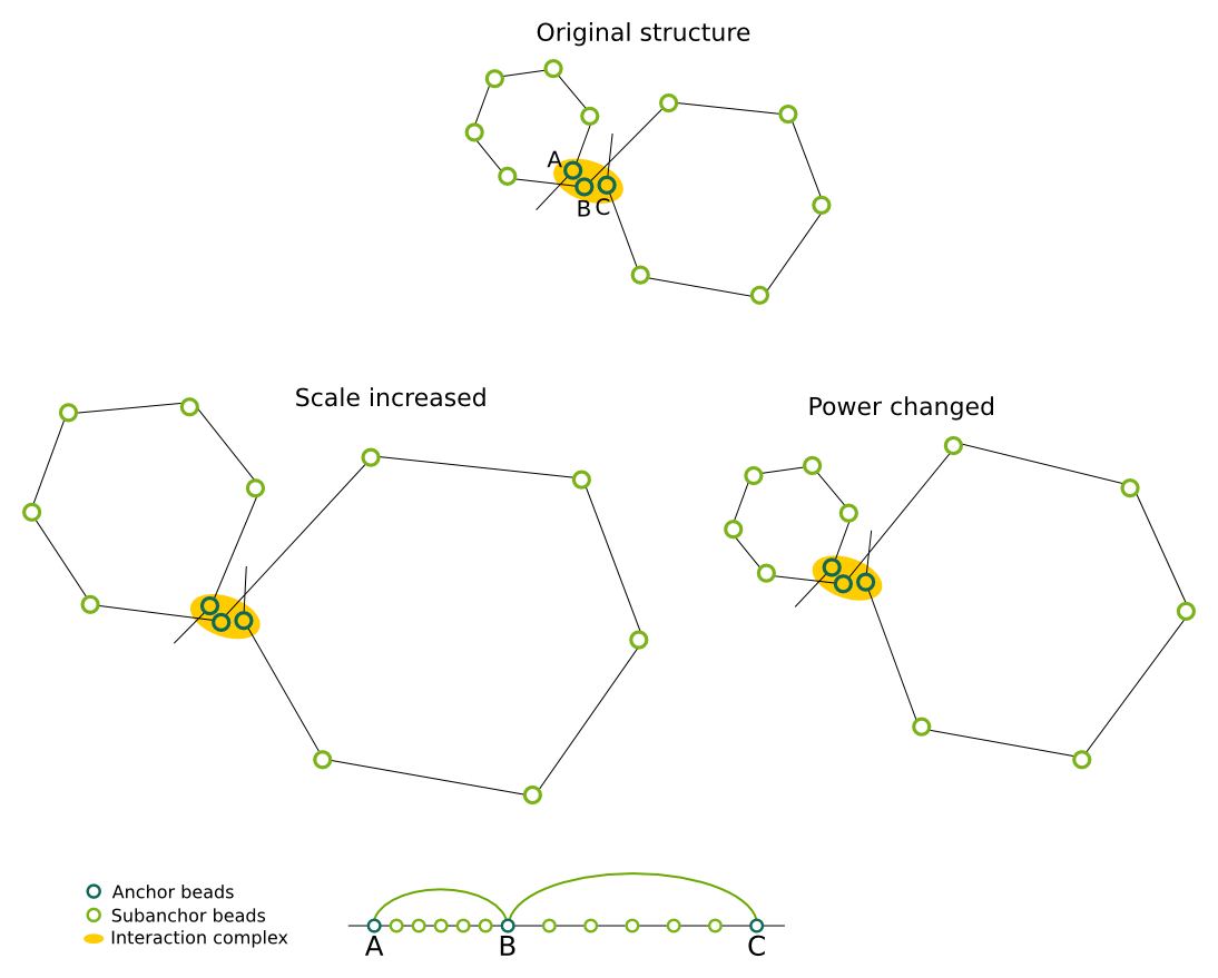
Anchor heatmaps
The distance between interacting anchors is approximated by the strength of the interaction. When anchor heatmaps are Enabled then the number of singleton interactions between the anchors is used to refine the distance. Weight describe the magnitude of the influence (range <0.0-1.0>).Subanchor heatmaps
Modelling on the subanchor level is primarily based on the distances and angles between beads, which results in a regular, circular loops. The shape of loops can be refined using the singleton interactions. Intuitively, if an increased number of interactions between two loops is observed, then they might be preferentially location in a closer proximity. Similarly, a pattern of singleton interactions within a single loop can be analyzed, which may serve to refine a shape of a particular loop, as presented on a picture below. The effect the singletons have on the subanchor heatmaps is described by these parameters. The single most important setting (besides of Enable, which turn this feature on/off) is Weight (range <0.0-1.0>), which denotes the strength of the effect the singletons will have. Weight describe the magnitude of the influence (range <0.0-1.0>). Steps and Replicates denote how many times the algorithm calculating the relative singleton strengths is run, and how large ensemble is generated in every step.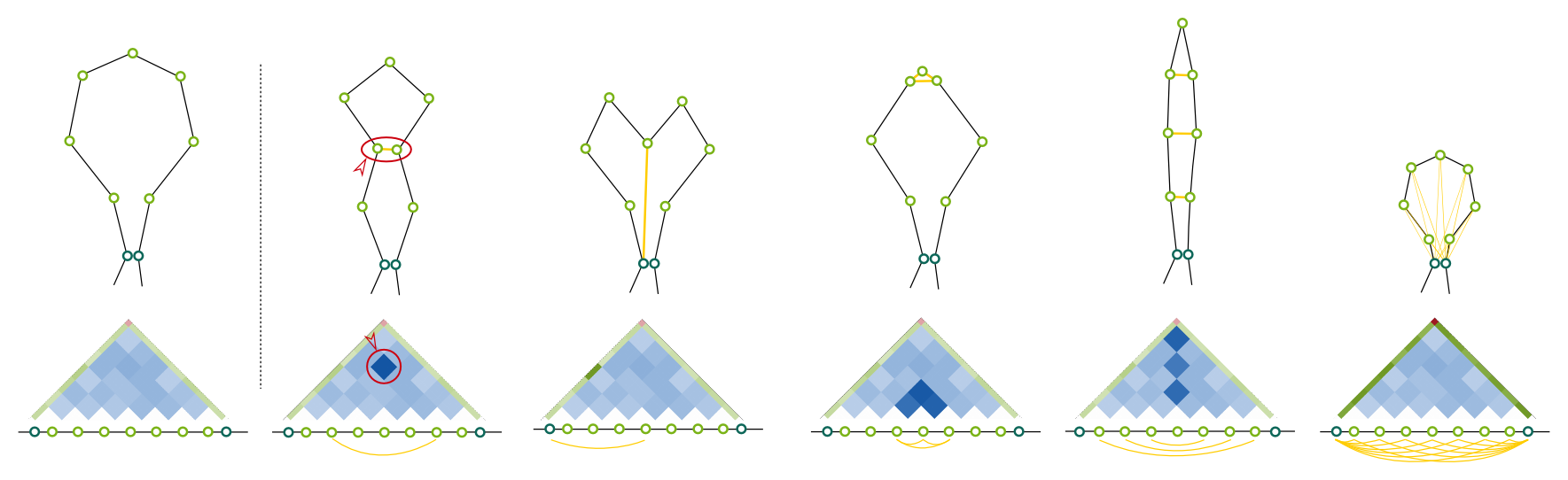
Modelling guidelines and common pitfalls
One of the crucial factors impacting the shape of the resulting structures is the split of genomic region into segments. Ideally, segments should reflect the underlying biological structures - topological domains. While domains are usually identified based on the aggregated contact maps (which would mostly correspond to singletons in case of ChIA-PET data) for our heuristic splits-finding algorithm we use PET clusters alone. This stems from the observation that strong interactions should appear mostly within domains, which was confirmed by our analysis (ie. segments based on PET clusters are very similar to the ones that can be deducted from singleton heatmaps).
In the current version we don't allow for displaying heatmaps in the data browser due to technical reasons. Still, users (specifically those submitting their own data) are encouraged to visually inspect the resulting segments and to compare them with heatmaps generated by other means, if possible.
While there is no single best split for a given data, there are some general guidelines that can be given. First, we prefer approximately megabase-sized segments - this is for both practical and theoretical reasons. Practically speaking, topological domains length is usually of this order, and we want segments to correspond to domains. On the other hand, for the computational reasons it is convenient to have segments of similar length, and that are not very short (one of the reasons is that this makes the heatmap-related biases smaller). Of course, some of domains may be very short or very long. Below we provide a short description how such cases can be handled.
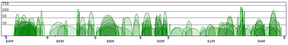
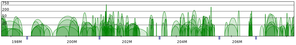
Sometimes PET clusters form clearly separated networks of interactions. More often the gaps between those
networks are not so large. Below 2 regions presenting both those cases are presented (note that for clarity
only CTCF interactions are showed).
Apart from the segment split 2 parameters have the largest impact on the resulting structures: frequency and genomic distance scales. Simply put, the former controls the size of structure on the segment level, while the latter - the size of genomic loops. To produce reasonable structures these 2 values need to be properly adjusted in relation to each other.
In more details, frequency scaling controls how the interaction frequency between segments
(i.e. the number of interactions between them) translates to the physical distance between the corresponding
beads. While the related Power parameter controls the rate the distance changes when interaction
frequency increases, Scale is simply a value that makes all the distances proportionally smaller or
bigger. If the value is too large the segment-level beads will be positioned very far from each other
resulting in a structure resembling a number of isolated small clumps (see figure below, left). On the other
extremum, if the value is too small the beads will be very close to each other, and the chromatin loops
from different segments will strongly overlap, to the point where the whole region looks like one large and
dense clump (below, right). Finally, when the parameters are adjusted properly we can obtain a structure
that
is more consistent with the current models of genome organization (below, center).


We note that in principle small datasets may be problematic for our algorithm, because the low-resolution structure is constructed based on the number of singleton interactions between segments. If the number of singletons is small then some of the segments may have no corresponding singletons, in which case we are not able to properly position the corresponding bead relative to others due to lack of information. Similarly, an input file with only a single PET cluster interaction could be problematic as well, as the resulting plots and 3D structure would not be very informative. For these reasons we require that there is at least 1 PET cluster positioned in every segment and at least 10 singletons anchored at every segment. Please note that it is difficult to define a lower limit guaranteeing that the simulation will be successful, so, if working with sparse datasets or very small regions, please be aware that specific combinations of clusters, singletons and segment boundaries may yield unexpected results. This, however, should not be the case if the real-life experimental data are used.
Please contact us if you have any troubles or questions concerning the method.
Limitations of 3D structure modelling method
Our method makes some assumptions about the chromatin organization and its relevance to the chromosome conformation capture (3C) based techniques, such as ChIA-PET and Hi-C. While there seem to be a general consensus as to the chromatin organization, specifically as to the existence and role of topological domains and chromatin loops, it it yet not clear how well these structures can be described using frequency interaction data.
Of particular problem is the relation between frequency of contacts between domains and spatial distances between them. While there were some functional relations suggested there are no clear experimental evidence for one or the other, on the contrary, it is suggested that different chromosomal regions may exhibit different scalings (the simplest example being eu- and heterochromatin). Currently our method support the inverse power law relationship. It does not currently allow for defining different scalings for different regions, but we are working in this direction. The default parameters were chosen based on our analysis (this will be reported elsewhere) and should work well in a typical case, but they may not be suitable for all the data. Below we present some simple examples of how one can adjust the parameters to produce a reasonable structures, but users are encouraged.
One should also be aware that both ChIA-PET and Hi-C data are population based, ie. the data is generated from millions of cells. Thus, a single model created based on that data does not represent a true conformation exhibited by a particular cell, but rather an average over the whole cell population. There are 2 main ways of dealing with this problem. The first is to treat the single resulting structure as a consensus model that represents the general shape. Thus the structural features need to be interpreted as the general tendencies of the population rather than a strict description of a chromatin. In the second approach one tries to create an ensemble of structures which may better reflect the possible cell subpopulations. Both methods have their advantages and limitations, and the best approach may depend on the ultimate goal of the analysis. In our case we are concerned more with the general landscape of the genome organization, and thus in our method we the consensus approach.
A more detailed discussion of these (and some other issues related to the interaction frequency data) can be found for example in [Lajoie et al, The Hitchhiker’s guide to Hi-C analysis: Practical guidelines, Methods, 2015].
Structural variation-driven alterations of chromatin spatial architecture
In 2.0 version of 3D-GNOME we applied an algorithm for modeling changes of the genome topology by removing and creating contacts between chromatin interaction anchors based on genetic alterations introduced by SVs. When given a set of SVs present in other lymphoblastoid genomes, it applies a series of simple rules to recover their individualized chromatin interaction patterns from the reference data. The resulting genomic interactions are then passed to the 3D structure modeling engine to build 3D models of individualized chromatin structures. Of note, while GM12878 ChIA-PET data is set as the reference for modeling 3D genomes of the samples genotyped by the 1000 Genomes Consortium, in principle any genomic interaction data can be used as the reference. The method acts on the following types of SVs: deletions, duplications, insertions and inversions. SV-driven modelling by the web server is described at Tutorial. The method was described in detail here.Deletions
Deletion removes all anchors within its scope, and therefore all the interactions they form with other anchors. Loops directly adjacent to the introduced deletion are elongated or shortened depending on the interaction pattern and size of the deletion. A deletion, which partially or completely overlaps the outermost anchor of a particular CCD, removes its boundary and merges it with the genomic region on the other side of the boundary. You can see an example here.Duplications and Multiallelic Copy Number Variants
Interactions that reside entirely in the duplicated region are repeated as a whole and introduced adjacently downstream in the genomic sequence. Similarly, a new copy of an anchor is created downstream from the original anchor. The original anchor maintains only the upstream interactions it formed before being duplicated. The downstream interactions are in turn connected to the duplicated anchor instead of the original one. Regarding CTCF mediated interactions, if the original anchor is lacking downstream contacts, naturally there are no interactions that the duplicated anchor could take over. In such cases, the algorithm finds the closest CTCF anchor with which it can create a convergent loop and connects them. This strategy reflects the currently assumed mechanism of CTCF-mediated chromatin loop formation, known as extrusion (19). According to this model, chromatin is pulled through the ring-shaped cohesin complex until the cohesin ring stops at an obstacle larger than the ring lumen. In this model, these obstacles correspond to CTCF proteins bound to the DNA motifs on the opposite DNA strands. Furthermore, if a duplication expands over a CCD boundary, parts of the CCDs, placed at the breakpoint after duplication, are fused. On top of having a direct impact on interacting loci, duplications can also increase the lengths of chromatin-loop spanning the duplicated regions. The effects of Multiallelic Copy Number Variants (mCNVs) are introduced in the 3D genome by performing multiple duplications or deletions. You can see an example here.Insertions
Inserted sequences are scanned for CTCF motifs using the PFM matrix. If a motif is found, the algorithm treats it as a new CTCF anchor and finds the closest anchor with which it can create a convergent loop. You can see an example here.Inversion
The algorithm reverses the directionality of the anchors affected by the inversion and removes all original contacts they formed. Next, it matches each of these anchors with the closest anchor of opposite orientation to create a convergent loop. If the considered anchors correspond to protein factors that do not bind any specific DNA motifs or if the orientation of the motifs they bind is irrelevant for the loop formation, the algorithm links such anchors with the closest ones, regardless of their directionality. If as a result of inversion, the algorithm links anchors from adjacent CCDs, the boundary between them is removed and the CCDs are merged. You can see an example here.Running time of simulation - examples
| region size | CTCF | CTCF, SVs | CTCF+RNAPII | CTCF+RNAPII, SVs |
|---|---|---|---|---|
| 1MB | 0:30s | <2 min | 2:30 min | 7 min |
| 2MB | 0:30s | <2 min | 3:15 min | 10 min |
| 5MB | 0:30s | 2 min | 3:15 min | 12:30 min |
| 48.1MB - chr21 | 3 min | 10 min | 8:30 min | 1 h |
FAQ
-
What are singletons and clusters?
Our modelling is based on ChIA-PET data, and the terms singletons and PET clusters denote the interactions that appeared only once (or only a very small number of times) and that appeared very frequently in the dataset obtained from the experiment, respectively. The basic interpretation is that PET clusters represent very confident, strong interactions, and thus can be used to identify chromatin loops, while singletons, which are not so confident (but are much more abundant) can be used to infer the spatial relationship between different contact domains, chromatin loops, or loci on a particular chromatin loops.
-
Why some of the singletons have high frequency?
In our dataset for an interaction to be classified as a cluster it must fulfill a number of requirements:
- Frequency at least 4
- Containing a CTCF motif sequence at both ends
- CTCF motifs oriented toward each other (convergent orientation) or in the same direction (tandem orientation)
- Colocalized cohesin peaks at both ends
-
Do I need to use ChIA-PET data?
No. While our modelling was designed specifically for the ChIA-PET in principle you can use any source of interaction frequency data, as long as you can identify weak and strong interactions.
-
Can I use Hi-C data for the simulation?
Yes, you can. You should supply your Hi-C interactions as singletons. To identify clusters you should perform loops calling.
-
How long should the computations take?
It well depends on the number of interactions in the selected region and whether the user wants to modify interactions by SVs or not. You can see the estimation of computation time here. Computation times depend on the number of protein factors (CTCF, or CTCF together with RNAPII) used for simulation and whether it involves SV-driven modeling. These times were measured when the job queue was empty, therefore it may take longer if the request needs to wait in a queue. Note that the default settings were used for the calculations, and some of the settings (particularly "Steps" options and enabling the subanchor heatmaps) and number of samples with the SVs list may impact the computation time significantly.
Note the maximal running time (ie. since the status changed to "Started") is set to 48 hours, after which jobs are killed. Please let us know if your computations take much longer than expected or if you need to increase the time limit.
-
What is the data format?
Please see Submitting custom data section
-
What is the default dataset?
By default we use the original dataset that was used in our recent publication (Tang et al, CTCF-Mediated Human 3D Genome Architecture Reveals Chromatin Topology for Transcription, Cell, 2015). This dataset contains 30 714 highly confident PET clusters with convergent or tandem CTCF motifs orientation, 100261 RNAPII clusters and 10 479 226 singletons (including 10 430 481 true singletons [frequency < 4] and 48 745 interaction with frequency >3, but without a CTCF motif, an incorrect CTCF motif orientation or without the corresponding cohesin peak).
This dataset is available here. The default SVs data are sourced from the catalogue of SVs identified by the 1000 Genomes Consortium for 2,504 genomes and is available here: The 1000 Genome Project (Phase 3). -
Is the modeling software available?
Yes, the modeling software we use is publicly available.